Mike Schaeffer's Blog

At my job, we use Excel extensively to keep track of software testing progress. One typical use is to maintain a list of features to be tested, along with their current pass/fail statuses and an attempt at a rough subdivision into functional areas. Excel's AutoFilter then makes it easy to ask questions like "show me all failed tests relating to function block scheduling."

This works really well as long as "function block scheduling" is one of the categories into which you've subdivided your features list. If it's not, you have to get a little creative to filter your list. One approach to this problem I've found useful is filtering based on columns populated with a formula similar to this:

=IF(ISERROR(SEARCH($K$5,K6)),"No","Yes")

If column K contains feature descriptions, this formula returns "Yes" is the description matches the search string in K5 and "No", otherwise. Filtering based on this formula makes it possible to display every list item whose description matches a word. If there is more than one column to search, you can use string concatenation to aggregate the columns together:

=IF(ISERROR(SEARCH($K$5,K6&L6&M6)),"No","Yes")

So, why the name apropos? Follow this link.

David Gainer has Summarized a a number of new conditional formatting rules in Excel 12, over on the Excel 12 blog. These rules were designed to "make a greater number of scenarios possible without needing to write formulas." In other words, all these scenarios have simple solutions directly visible in the Excel 12 UI.

Well, if you can't wait for Excel 12, Excel is pretty darned powerful as it is, and as Mr. Gainer states: most of these scenarios have formula-based approaches that work right now. Here are some of the approaches for current versions of Excel:

• With data bars, color scales, or icons based on the numeric value in the cell, percentages, percentiles, or a formula. See the posts on data bars, color scales, and icon sets for more information on each of these. - This approach to 'databars' generalizes to formula-based scaling, although it's not as pretty, not a color scale, and not an icon set.
• Containing, not containing, beginning with, or ending with specific text. For example, highlighting parts containing certain characters in a parts catalog. - Use a formula: a lot of these conditions can be tested using FIND: =FIND(string, A1)=1, checks for parts that begin with string, for example.
• Containing dates that match dynamic conditions like yesterday, today, tomorrow, in the last 7 days, last week, this week, next week, last month, this month, next month. For example, highlight all items dated yesterday. The great part about these conditions is that Excel handles calculating the date based on the system clock, so the user doesn.t need to worry about updating the condition. - Use a formula: the system date is available via NOW(), and Excel offers plenty of date arithmetic functions to check for specific conditions.
• That are blank or that are non-blank. - Use a formula: =ISBLANK(A1) or =NOT(ISBLANK(A1))
• That have errors or that do not have errors. - Use a formula: =ISERROR(A1) or =NOT(ISERROR(A1))
• That are in the top n of a selected range (where n is whatever number you want) OR that are in the top n percent of a selected range (again, where n is adjustable). For example, highlighting the top 10 investment returns in a table of 1,000 investments. - Use a formula: =RANK(A1, range) > n.
• Cells that have the bottom n values OR cells that are the bottom n percent of a selected range. - Use a formula: `=RANK(A1, range)n`.
• Cells that are above average, below average, equal to or above average, equal to or below average, 1 standard deviation above, 1 standard deviation below, 2 standard deviations above, 2 standard deviations below, 3 standard deviations above, 3 standard deviations below a selected range. - This type of thing can be solved using a particular form of formula: =A1<(AVERAGE(ange)-n*STDEV(range)) or =A1>(AVERAGE(ange)+n*STDEV(range)). For large ranges, it probably makes sense to move the computation of AVERAGE and STDEV into a cell, and have the conditional format reference (with an absolute reference) that cell.
• Cells that are duplicate values or, conversely, cells that are unique values. - Use a formula: =COUNTIF(range, A1)=1 or =COUNTIF(range, A1)>1. Ensure that the range you use in the formula has an absolute address. If your range is sorted on the 'key' field, you can use this style of formula: =A1<>A2. This can be much, much faster, particularly for large tables. (For the Comp. Sci. types it's O(N), rather than O(N² ), once you have sorted data.)
• Based on comparisons between two columns in tables. For example, highlight values where values in the .Actual Sales. column are less than in the .Sales Target. column. - Use a conditional format formula: =A1<B1. Apply it to the entire column you want shaded, and Excel will evaluate the seperately for each cell. The cell references in the format formula are relative to the current cell in the selected range. The current cell is the cell in the range that is not highlighted (but is surrounded by a selection border), and can be moved around the four corners of the range with Control+. (period).
• When working with tables, we have also made it easy to format the entire row based on the results of a condition. - Relative formulas can be made to do this: select an entire range, and define a conditional formula using absolute column addresses (ie: =$a1). Excel evaluates the format formula for each cell in the range, and since the column addresses are absolute, each cell in a row will pull from the came columns. Therefore, each cell in a row will share the same conditional format, which is what we want.

Based on this, you don't have to wait for Excel 12 to get a lot of these features, you just have to wait for Excel 12 if you want Excel to do it for you automatically. My suggestion would be to learn how to use conditional formatting formulas, but I tend to be "here's how to fish" kind of guy more than a "here's a fish" kind of guy.

I suspected as much, but Excel has a way to duplicate my UDF using Excel formulas.

=REPT("█",A1) & REPT("▌",ROUND(FLOOR(A1,1),0))

That formula evaluates to a bar of length A1 units, rounded to the nearest 0.5. Rescaling can be done in another cell. If you're interested in a bar that can be right-justified, you can use this:

=REPT("▐",ROUND(A1-FLOOR(A1,1),0)) & REPT("█",A1)

The trickiest part about this is getting the block characters into the formula. For that, I reccomend using the Windows Character Map.

Qualitatively compared to VBA, this method requires more logic to be represented in the spreadsheet: that adds compelxity for readers and makes it tricker to set up than the VBA. On the other hand, it avoids the performance hit of calling UDF and the requirement that the spreadsheet contain a macro. I honestly don't know which is better style, but can say that this would be a perfect time to use a paramaterized range name (if Excel had such a thing).

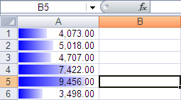
Microsoft has just announced a cool new feature on the Excel 12 blog: the databar. I think a picture can explain it better than I can:

Note from August 2025: This picture was formerly linked from Microsoft's Excel 12 blog, which borrowed it from another site. All that's gone now, but thanks to the magic of the Wayback Machine, I've found a copy to host locally.

This will be a nice way to look for trends/outliers, but I can also see it being useful for tracking parallel completion percentages in status reports, etc. Of the Excel 12 features announced so far, this is the one that I'm the most excited about. Of course, it's also the one that's easiest to approximate in Excel <12. Andrew has an approach using Autoshapes on his blog, and I'm going to present a slightly different approach.

IMO, his approach looks a lot better, this approach has the benefit of updating automatically. Pick your poison. It all centers around this little UDF:

Option Explicit

Function GraphBar(x As Double, _
                  Low As Double, _
                  High As Double, _
                  ScaleTo As Double) As String

    x = ((x - Low) / (High - Low)) * ScaleTo

    Dim i As Integer

    Dim blockFull As String
    Dim blockHalf As String

    blockFull = ChrW(9608)
    blockHalf = ChrW(9612)

    GraphBar = ""

    For i = 1 To Fix(x)
        GraphBar = GraphBar + blockFull
    Next

    If x - Fix(x) > 0.5 Then
        GraphBar = GraphBar + blockHalf
    End If
End Function

This isn't rocket science: all it does is rescale x from the range [Low, High] to the range [0.0, ScaleTo]. Then, it strings together that many Chrw(9608)'s, followed by a Chrw(9612), if the scaled value's fractional part is >0.5. The trick in this is that Chrw(9608) and Chrw(9612) are VBA expressions that produce the the Unicode equivalent of the old line drawing characters IBM put in the original PC [1]. 9608 is a full box ("█"), 9612 is a half box on the left ("▌"). The result of this function ends up being a string that (when displayed as Arial) looks like a horizontal bar. ("████▌"). Put a few of those in adjacent cells, and you get this:

The formula in C2 (and filled down) is =GraphBar(B2,MIN(B$2:B$8),MAX(B$2:B$8),5). The MIN and MAX set the scale, the 5 sets the maximum length of a bar. The maximum length, font size, column width can be tweaked to produce a reasonably attractive result, although I do reccomend using vertical centering.

If you want to get a little fancier, conditional formatting works on plot cells...

...whitespace can possibly improve the appearance...

...and this technique can scale.

1] (The original PC didn't have standard graphics, it was an option. If you bought the monochrome, non-graphics, video board, characters like this were as close as you could get to a bar chart.)